The program

The cosmoscope is a computer tool that allows ordering and accounting for astrological variables in a large number of natal charts of people with some common characteristic such as professions, life experiences or events, behavioral tendencies, outstanding skills, pathologies, etc.

It operates by comparing the frequency of the variables observed in the study population (FO) with the frequency of the variables in a control population (FN), providing the key data, which is the relative frequency (Fr). The RF highlights the variables that distinguish astrologically from the studied population.

The control group is automatically generated by the same program by preparing a fictitious day-by-day list of all the people born within the same time interval in which the subjects of the study population are included. Considering this circumstance, it is necessary that the study population is more or less uniformly distributed over a period of time.

Astrological variables in principle are planets in signs, planets in houses and aspects between planets.

DATA:

Name of the list or characteristic that identifies the population to be studied

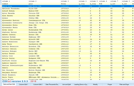
List of names with date, GMT, country, city, latitude and longitude

interval of dates within which are all the births on the list

Define option with or without birth time

planetary orbs. The program works with defined orbs which can be changed to the investigator’s taste.

RESULTS:

1. List of all names with the planetary positions and houses

2. Frequency table Planets in signs

2.2 – Frequency observed in /12 (for most will be approximately 1)

2.1 -Frequency observed in absolute values

2.3 – Normal frequency distribution[1] /12

2.4 – Relative frequency distribution (observed frequency/normal frequency)

3. Table of frequencies of planets in solar houses

3.1 -Frequency observed in absolute values

3.2 – Frequency observed in /12

3.3 – Normal frequency distribution /12

3.4 – Relative frequency distribution (observed frequency/normal frequency)

4. Frequency table Planets in houses. (optional)

Step 4 can be done with various house systems.

4.1 -Frequency observed in absolute values

4.2 – Frequency observed in /12

5. Matrix of Major Aspects.

Table that includes for each pair of planets twelve possible aspects. The separative aspects are differentiated from the approximate aspects, thus giving rise to the twelve. Special tables are included for the Mercury Sun and Venus Sol aspects.

5.1 -Frequencies observed in absolute values

5.2 – Frequencies observed in %

5.3 – Normal frequencies calculated within the entered date range

5.4 – Final table with observed frequencies / normal frequencies

Table of aspects for each pair of planets

Aspects should be understood by rotating counterclockwise starting from the conjunction

>	n	C	b	?
Z	A G			x
>	n	C	b	?

6. Table of frequencies of Ascendants and MC in signs (optional)

Can be made for various house systems

6.2 – Frequency observed in /12

6.1 -Frequency observed in absolute values

For each pair of planets, for example Sun Mars, there is a table of aspects that contains the following information:

7. Mercury cycle table.

It is a table that presents the positions of mercury during its synodium cycle, it contains the two conjunctions, the two maximum elongations both the western and the eastern and the intermediate spaces. Mercury rotates around the sun anti-clockwise.

Late between 6th and 18th	space between V is 70until it approaches 18º from the sun	Late Max-Separation Western Promethean 70< V < 50	Space between the station until V grows to 50	From the conjunction to the retrograde to direct station
AZD Orbe ± 6º D direct behind the sun	AD			AZD Orb ± 6º D Retrograde in front of the sun
Advance between 6th and 18th	space from when you start to move more than 18º until the V is reduced to 70	Advance max-separation oriental epimetheic 70< V < 50	space between that v = 50 until it is reduced to zero	From direct to retrograde station to conjunction V =0

Explanation Table Mercury Cycle

Advance refers to the fact that it is at a zodiac degree later than the degree of the Sun, it is equivalent to an Eastern Mercury or an evening Mercury.

Backward refers to the fact that it is at a zodiac degree further back than the degree of the Sun, it is equivalent to a Western Mercury or a morning mercury.

8. Special table to analyze the Venus cycle.

Table with the different positions of Venus in its synodic cycle. It contains the two conjunctions, the two maximum elongations both the western and the eastern, the four types of semi-sextiles and the intermediate spaces. The meanings of Venus in each of these positions are very little studied so far.

F > A Orb ± 3rd	mean value	Delay Max. distance	mean value	F > A Orb ± 3rd
Backed between 27º and 6º	f to			Late between 6th and 27th
f z a orb ± 6º F direct behind the sun				f z a orb ± 6º f retrograde in front of the sun
Advance between 6th and 27th				Advance between 27th and 6th
F > A Orb ± 3rd	mean value	advance max. distance	mean value	F > A Orb ± 3rd

9. Table of grouped aspects

This table contains three groups:

AAA harmonic associative aspects that are conjunctions, trines and sextiles.

sum of the previous two.

Disjunctive associative aspects AAD that are oppositions and quadratures.

For each of the groups, they show the percentages of the relative frequency found, the frequency in the normal population and the relative frequency or quotient between the previous two.

10. Graphics of the profile and anti profile of the study population.

The first profile contains planets in signs, ASC in signs and MC in signs

A second profile contains planets in houses

The graph consists of a circle divided into 12 parts associated with the twelve signs or the houses. In each sector, the planets that have obtained a high frequency for that position and the low frequencies in the anti-profile are placed.

Considerations on how to measure frequencies

The relative frequency of all the variables studied refers to the quotient between the frequency found in the study population and the normal frequency. Finally, that is the fact that interests us. In this regard we will use the following levels.